Alazartech Acquisition card

Introduction

Card developed by Alazartech for the acquisition of signals: Alazartech website. It is used to acquire signals, and to analyse them to perform FFT, PSD or a Rabi experiment.

Installation

The code for the control of Alazartech acquisition cards is part of PyHegel, to be installed following the instructions on PyHegel repository. The code is in the instruments module of PyHegel, under the name ‘Alazartech.py’. You can detect all the Alazartech acquisition cards connected with the computer using the find_all_Alazartech() function.

>>> instruments.find_all_Alazartech()

If cards are connected together, they form a system. The function returns a dictionary having for keys the labels of the system and for values a tuple with the number of cards in the system and a new dictionary with keys the labels of the card in the system and values the main information about the card. All cards are represented by the id number of their system and their id in this system. You can connect with any cards detected using instruments.find_all_Alazartech() by using the function instruments.ATSBoard(systemId=1, boardId=1)()

>>> ats = instruments.ATSBoard()

In our case, we have only one card Alazartech, so its systemId and boardId are both equal to 1. If no cards are detected using instruments.find_all_Alazartech(), the installation of the card should be checked. First, check if the card is correctly wired on the computer, then check if its pilots are well installed and finally if the SDK version should not be updated. Information about the installation of the card is found on the Alazartech website, and information about the version of the SDK and Driver are obtained using instruments.find_all_Alazartech().

Overview of the functionalities

Working with PyHegel

From the iPython interface of PyHegel, you can create an Alazartech card instrument using instruments.ATSBoard(). This instrument is an instance of the Python class instruments.ATSBoard. In this instance, some devices are defined, that are interactive attributes of the instrument. In the following, all the devices of instruments.ATSBoard() are written as device. The minimum function of devices is to store data. The value of a device device is obtained via its method get(). The get() method is defined in pyHegel and has many features, including the possibility to write the data in a file by defining a filename in the filename option. The file is saved in the “.txt” format, but it can be saved in another format by defining it in the bin option. See PyHegel documentation, run get? or get?? in the PyHegel console to see the get options. Generally speaking, you can access the description of any device by running device? and see the source code of the device by running device??.

>>> ats = instruments.ATSBoard()  # ats is an instrument
>>> ats.acquisition_length_sec.get()  # print the value of the device acquisition_length_sec
>>> get ats.acquisition_length_sec, filename="acquisition_length_sec.txt"  # print the value of the device acquisition_length_sec and store it in a .txt file
>>> ats.acquisition_length_sec?  # see documentation associated with device acquisition_length_sec

All the devices and their value can be obtained by running ipython(). The value of certain devices can be changed interactively using the :py:func:set method.

>>> set ats.acquisition_length_sec, 1e-3  # device acquisition_length_sec now stores the value 1e-3
>>> ats.acquisition_length_sec.set(1e-3)  # same operation

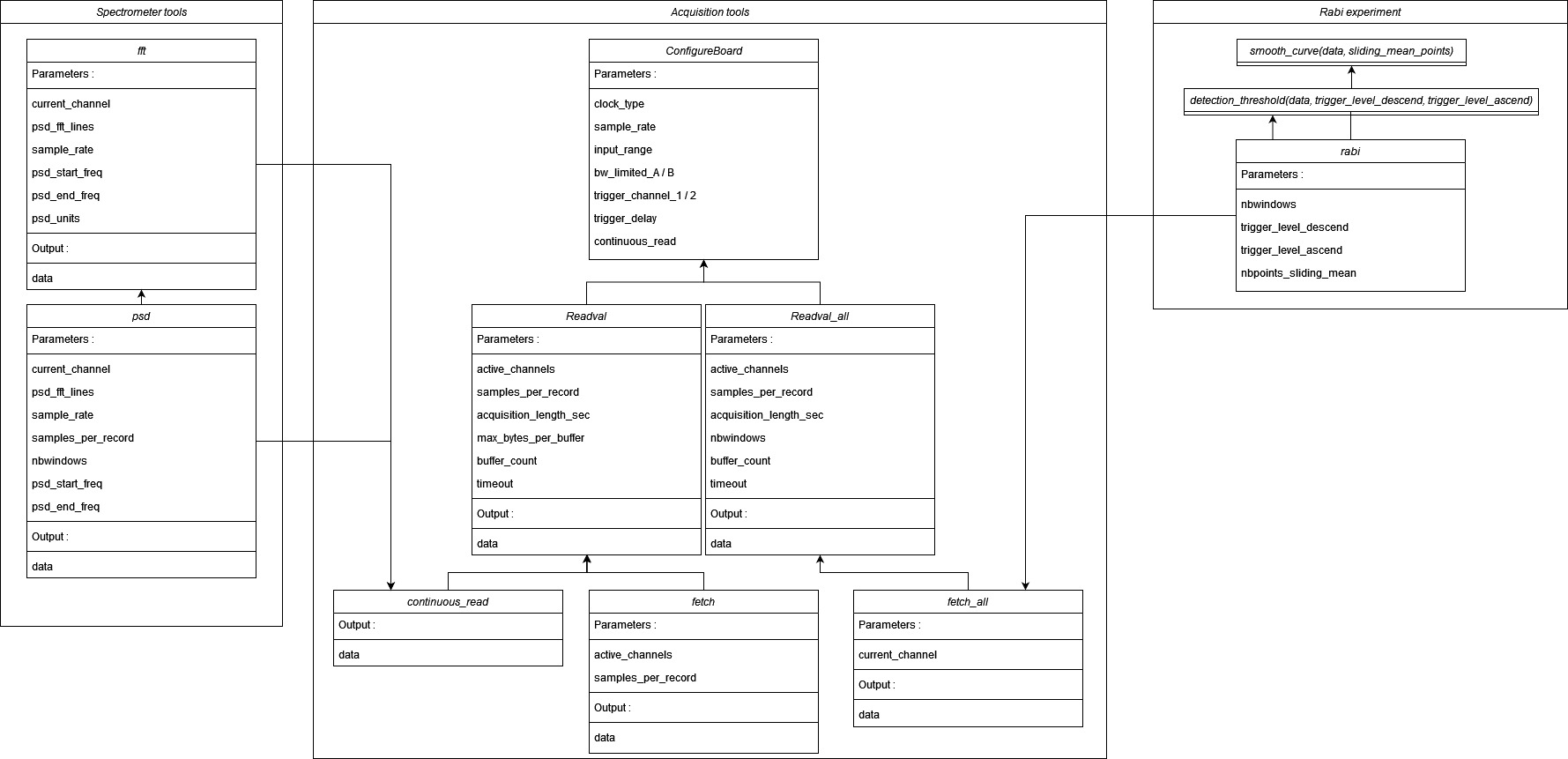
Devices and functionalities of the card

The main functionality of the card is to acquire signals. Acquisition are of different types, see the acquisition types), and are defined by their duration acquisition_length_sec, the number of points per acquisition samples_per_record and the sample rate sample_rate. You can acquire up to two streams of data and trigger using these channels or an external signal (see acquisition ports). The acquisitions are performed as on an oscilloscope and you need to define the size of the screen with input_range, and the mode of the screen with acquisition_mode. You can also modify some inner parameters of the acquisition.

The card can also be used to post-process signals. The FFT or the PSD of any acquired signal can be made using instruments.ATSBoard.make_fft() or instruments.ATSBoard.make_psd(). The FFT or the PSD of a channel defined in current_channel can be directly performed using fft or psd. The main parameters for these post-processing are the number of points taken to perform FFT psd_fft_lines, the sample rate, the unit of the output psd_units and the starting and ending frequencies at which the FFT/PSD should be shown, psd_start_freq and psd_end_freq.

It can also be used to analyse the results of a Rabi experiment using rabi. After acquiring nbwindows acquisitions, instruments.ATSBoard.detection_threshold() detects the times at which the signal crosses a threshold in a descending or ascending way (trigger_level_descend and trigger_level_ascend). It is possible to smooth curves using a sliding mean method involving nbpoints_sliding_mean points with instruments.ATSBoard.smooth_curve().

Acquiring signals

Acquisition ports

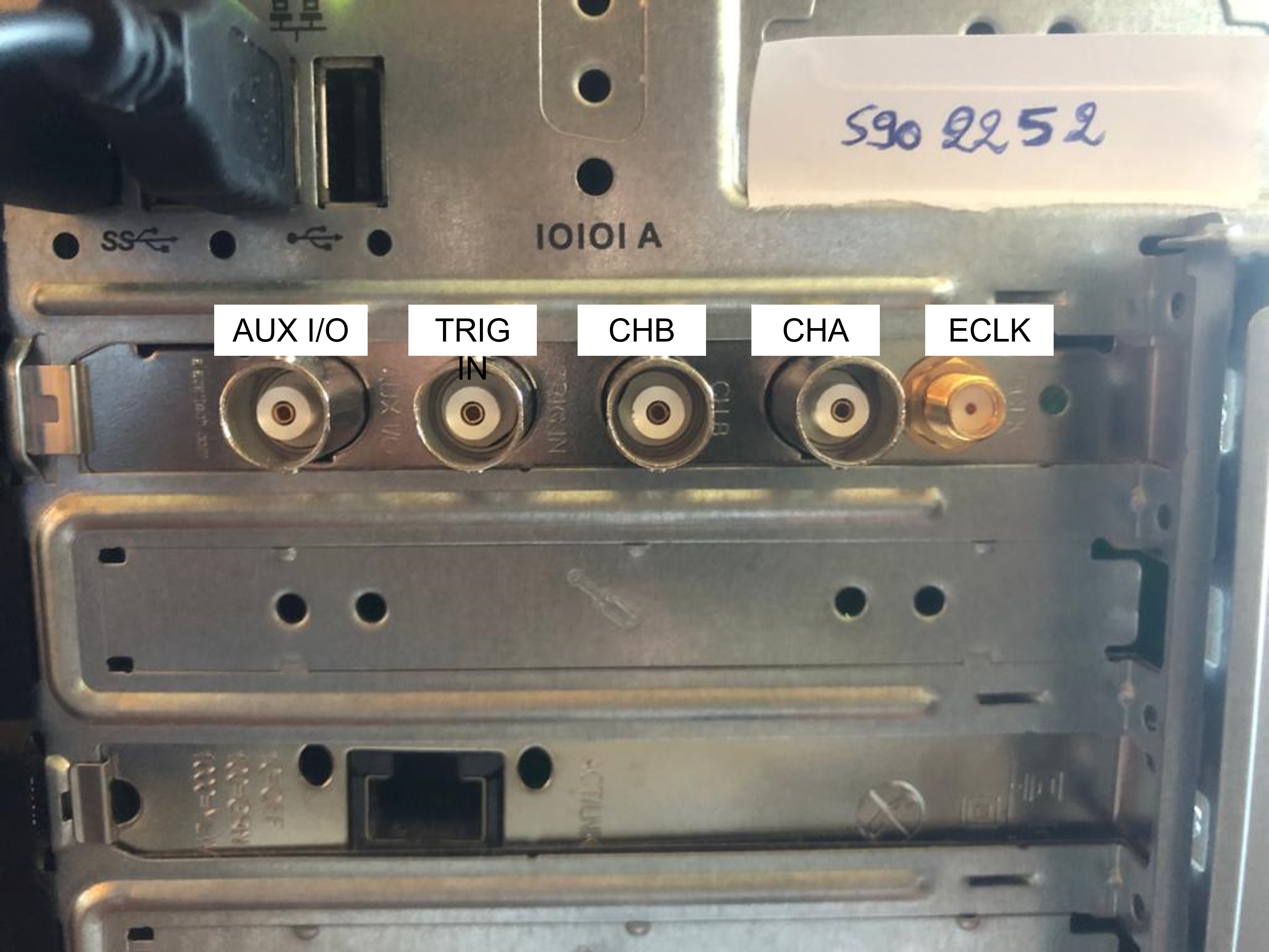
On the back of the Alazartech card, 5 ports can be connected with coaxial cables.

• The ports CHA & CHB acquire signals on Channel A and Channel B.

• the port TRIG IN is to receive a signal used to trigger acquisition of channel A and/or B.

• the AUX I/O port is to synchronize instruments by either supplying a 5V TTL-level signal or receiving a TTL-level input signal.

• the ECLK port is to acquire signals on channel A and/or B with a sample rate between 150 and 180 MHz in 1MHz step by receiving.

It is possible to acquire either channel A or channel B or both of them. The device active_channels defines a list of the channels to acquire. For each channel to acquire, trigger_channel_1 and trigger_channel_2 defines which port to use as a reference for the trigger operation, and trigger_level_1 and trigger_level_2 stores the level at which to trigger in mV. The acquisition can start when the signal reaches the trigger level in an ascending or descending way, which is defined in trigger_slope_1 and trigger_slope_2.

The internal clock of Alazartech cards enables the acquisitions to be performed only for certain sample rates. These sample rates depend on the acquisition card, but they range from 1KS/s to 4GS/s for the best cards. You can choose between using an internal clock INT and an external clock EXT by defining clock_type.

The AUX I/O port can be configured using aux_io_mode and aux_io_param.

Acquisition types

Three types of acquisition can be performed.

• readval.get() performs a trigger operation: it acquires the signal for a duration acquisition_length_sec at a sampling rate sampling_rate when the signal reaches a threshold current. fetch.get() works similarly. If an acquisition has already been performed for the channels defined in active_channels, it simply outputs the result of this acquisition. Otherwise, fetch.get() calls readval.get().

• readval_all.get() performs several trigger operation faster than by repeating readval.get(). The number of acquisitions is defined by device nbwindows and the channels to acquire are defined by active_channels. The function fetch_all.get() works similarly, except it only gets data for one channel, the current_channel. nbwindows is set to \(\lfloor \sqrt{n} \rfloor (\lfloor \sqrt{n} \rfloor + 1)\) if is not a square.

• continuous_read.get() acquires a signal right after being called. It calls readval.get() but with a trigger_mode set to Continuous instead of Triggered.

The sampling rate, the acquisition time and the number of points per records are related as \(sample\_rate * acquisition\_per\_second = samples\_per\_record\). sample_rate can only take some values, and a finer control can be obtained by using the ECLK port. Changing the sample rate impacts the number of samples per record without changing the duration of the acquisition. Changing the duration of the acquisition also impacts the number of samples per record without changing the sample rate.

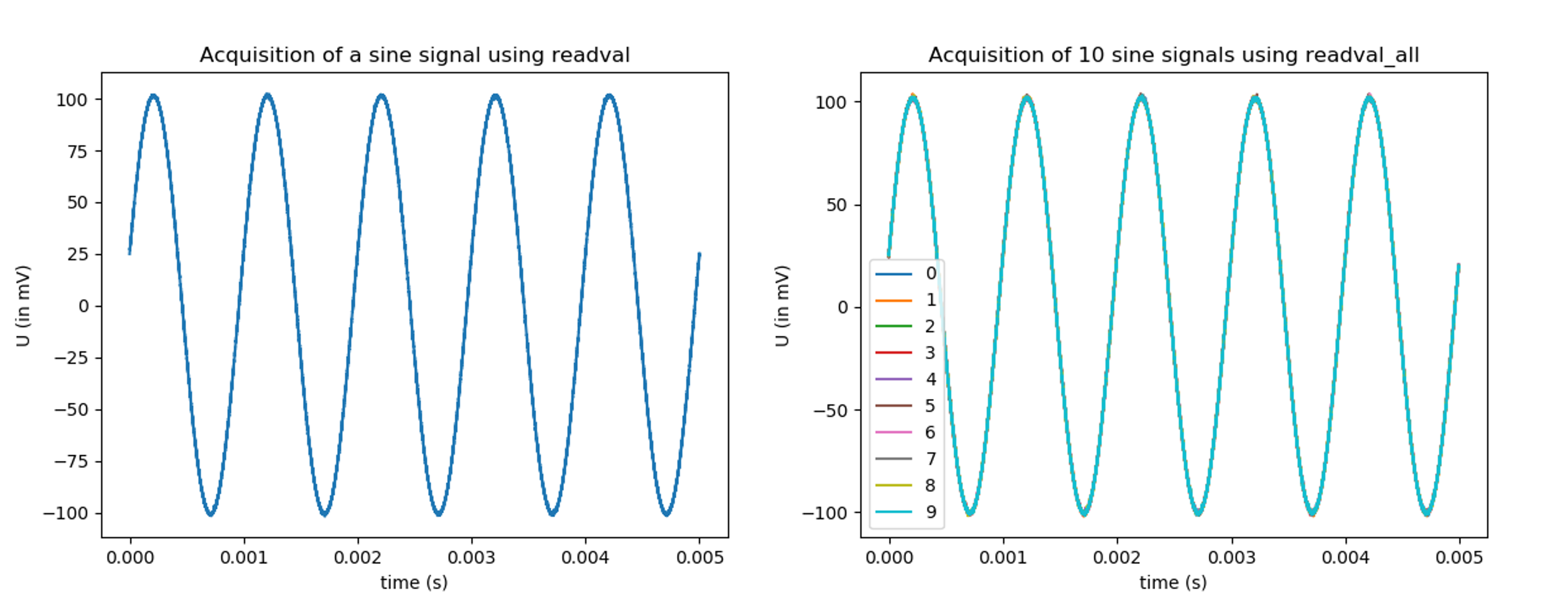
>>> ats = instruments.ATSBoard()
>>> set ats.trigger_level_1, 0
>>> set ats.sample_rate, 10e6
>>> set ats.acquisition_length_sec, 5e-3
>>> data = ats.readval.get()
>>> plot(data[0], data[1])

>>> set ats.nbwindows, 10
>>> data = ats.readval_all.get()
>>> for i in range(10):
...     plot(data[0], data[i+1])

>>> set ats.acquisition_length_sec, 1
>>> get ats.continuous_read

Structure of an acquisition

Before actually performing the acquisition, some operations have to be realized. The card should first be configured, which means that the sample_rate, the clock_type used for the sampling, the size of the screen input_range, the delay to trigger trigger_delay should be provided to the card, alongside information about the ports AUX I/O (aux_io_modes and aux_io_param), channel A (channel 1) and B (channel 2), that are the channel used to trigger trigger_channel_1/trigger_channel_2 , the level at which to trigger trigger_level_1/trigger_level_2, the slope for which to trigger (for an ascending or descending signal) trigger_slope_1 and trigger_slope_2, and the limit of the bandwith bw_limited_A/bw_limited_B. This configuration is performed in instruments.ATSBoard.ConfigureBoard(). When calling this function, the board is configured if the parameters have never been provided to the card or if one parameter was modified since the previous configuration (the inner attribute of the card _boardconfigured stores this data). This function is called at the begining of all the acquisition functions.

Once configured, the card performs an acquisition by filling DMA Buffers in its inner memory. The number of these DMA Buffers can be changed with the device buffer_count. In the Alazartech guide, it is adviced to have more than 2 DMA Buffers, and that having more than 10 DMA Buffers seem unnecessary. These DMA Buffers are defined by the number of bytes they contain. This number of bytes per DMA Buffer is derived from the number of samples per record samples_per_record, the maximum number of bytes per buffer max_bytes_per_buffer, the number of active_channels and the number of bytes per sample (defined in the attribute board_info with the key “BytesPerSample”).

In readval_all, the number of trigger operations to perform (defined in nbwindows) is redefined such that there is \(\lfloor\sqrt{nbwindows}\rfloor\) records in each of the \(\lfloor\sqrt{nbwindows}\rfloor\) buffers if the value of nbwindows is a square (\(\lfloor\sqrt{nbwindows}\rfloor+1\) buffers otherwise). Another condition for this device to work is that the value of samples_per_record should be a multiple of 128.

During an acquisition, the DMA Buffers are filled one after another and emptied in the same order in a dictionary data having keys the time t, and the channels A and B. This way, it is possible to use more buffers than the number of DMA Buffers. The acquisition is performed by the function waitAsyncBufferComplete(), that takes as parameter the address of the DMA Buffer to fill and a time after which to stop the acquisition, defined in the device timeout.

At the end of an acquisition, the data is re-written in an array with first column t, and second and/or third column A and/or B (depending on the active_channels). This way the data can be directly written in a file using the get() of PyHegel.

Performing the PSD/FFT of a Signal:

Fast Fourier Transform

The Fast Fourier Transform (FFT) of a signal having first column the time and second column the voltages of a signal can be performed using instruments.ATSBoard.make_fft(). The number of frequency points at which the FFT is computed is always equal to samples_per_record. It is described by another variable in order not to mix the temporal and frequency acquisitions psd_fft_lines. A FFT acquisition is also defined by psd_linewidth, that is, the frequency difference between two frequencies at which the FFT is computed. This quantity is the inverse of the duration of the acquisition (in seconds). With these two parameters the FFT is computed for frequencies ranging from 0 to \(\frac{sample\_rate}{2}\) (Nyquist criteria).

It is possible to ask for only a part of the FFT to be shown by modifying the range of the frequencies psd_span. If this range is smaller than \(\frac{sample\_rate}{2}\), it is possible to define the psd_start_freq, psd_center_freq or psd_end_freq (one defines the other as \(f_{end} = f_{start}+f_{span}\) and \(f_{end} = f_{center}+\frac{f_{span}}{2}\)) such that only the frequencies between psd_start_freq and psd_end_freq are shown. The values of these devices should always be such that \(f_{end} \leq \frac{sample\_rate}{2}\).

The units the FFT acquisition should be displayed can be in V or in dBV, and should be defined in psd_units. The device fft acquires a signal from current_channel and calls make_fft(). If the value of psd_units is not V or dBV it is set to V when calling make_fft(). make_psd calls make_fft() if psd_units is V or dBV. Analogously psd acquires a signal from current_channel and performs the psd by calling make_fft() if psd_units is V or dBV.

Power Spectral Density

The Power Spectral Density (PSD) of a signal is computed in instruments.ATSBoard.make_psd(), if the units defined in psd_units are defined as PSD units (V**2, V**2/Hz, V/sqrt(Hz)). The Welch method is used.

• The acquisition is cut in nbwindows of \(\lfloor\frac{NbSamples}{NbWindows}\rfloor\) points.

• Each sub-acquisition is multiplied by a window_function.

• Take the FFT of each result (number of points for the FFT defined by psd_fft_lines, under the condition that it is lower or equal to \(\lfloor\frac{NbSamples}{NbWindows}\rfloor\).

• Take the average of the square of FFTs. Output the data if the value of psd_units is V**2.

• Divide by the bandwith to obtain units in V**2/Hz. Take the square root of the result to obtain units in V/sqrt(Hz).

Performing a Rabi experiment

Description of a Rabi experiment

A Rabi experiment is composed of three stages. First, the gate voltage is high such that we are sure we load the quantum dot with an electron. After a long time, the atom is in its ground state. A microwave pulse of frequency \(\omega\) interacts with the electron during a time \(t_{Rabi}\) such that the electron is in its excited state with probability \(\cos(\omega t_{Rabi})^2\). During a second stage, we stop the microwave pulse and lower the gate voltage so that the energy of the electron is between the ground and excited state. If it is in the ground state, no current will be measured during this phase. If it is in the excited state, a current will be measured. During a third stage, the gate voltage is set low such that the electron is definitely out of the box. The whole experiment consists in repeating these three steps many times for various duration of the microwave pulse. For each \(t_{Rabi}\), we compute the number of acquisitions in which a current drop was measured and divide it by the number of iterations.

Acquiring a Rabi experiment

The rabi device performs nbwindows acquisitions of the current_channel one after another using fetch_all. Afterwards, these acquisitions are analyzed to extract the times at which the voltage goes above threshold_level_ascend or below threshold_level_descend. This extraction is performed by instruments.ATSBoard.detection_threshold(). It is possible to smooth the signal using a sliding mean filter instruments.ATSBoard.smooth_curve() before the detection of the thresholds. The number of points taken for the sliding mean is defined in sliding_mean_points. If this number is 0, then the detection is directly performed on the signal.

Tests & Performances

The time duration of any command on PyHegel can be computed by writing %time before the command. This way we measure the duration of the various acquisition tools (mean over 100 calls).

Time duration of some acquisition tools (mean over 100 calls)

readval, acquisition_length_sec=5e-3	readval_all, acquisition_length_sec=5e-3, nbwindows=100	continuous_read, acquisition_length_sec=5e-3	continuous_read, acquisition_length_sec=1
0.16s	10.58s	0.182s	1.43s

It can be noticed that it is faster to call readvall_all with nbwindows set to 100 (takes 10.58s) than to call readval 100 times (takes 16s). The post-processing doesn’t take much more time.

Time duration of some post-processing tools, for a sample rate of 10MHz

rabi, acquisition_length_sec=5e-3, nbwindows=100, sliding_mean_points=0	rabi, acquisition_length_sec=5e-3, nbwindows=100, sliding_mean_points=10	fft, acquisition_length_sec=1	psd, acquisition_length_sec=1
10.59s	10.60s	1.69s	2.10s